Forecasts Are More Accurate for Individual Items Than for Groups or Families of Items.
Topic four Part 2: Applications of Supply and Need
4.7 Taxes and Subsidies
Learning Objectives
Past the terminate of this section, yous volition be able to:
- Distinguish between legal and economic tax incidence
- Know how to represent taxes by shifting the curve and the wedge method
- Understand the quantity and price affect from a taxation
- Describe why both taxes and subsidies cause deadweight loss
Taxes are not the most popular policy, but they are often necessary. We will look at 2 methods to understand how taxes affect the market: by shifting the curve and using the wedge method. First, we must examine the departure between legal tax incidence and economic tax incidence.
Legal versus Economical Tax Incidence
When the government sets a tax, information technology must decide whether to levy the tax on the producers or the consumers. This is calledlegal tax incidence. The most well-known taxes are ones levied on the consumer, such equally Authorities Sales Taxation (GST) and Provincial Sales Tax (PST). The government also sets taxes on producers, such as the gas tax, which cuts into their profits. The legal incidence of the tax is really irrelevant when determining who is impacted by the tax. When the authorities levies a gas tax, the producers will pass some of these costs on equally an increased price. Likewise, a tax on consumers will ultimately decrease quantity demanded and reduce producer surplus. This is because the economic tax incidence, or who really pays in the new equilibrium for the incidence of the taxation, is based on how the market responds to the price change – non on legal incidence.
Revenue enhancement – Shifting the Curve
In Topic iii, we determined that the supply bend was derived from a firm'south Marginal Cost and that shifts in the supply bend were caused by whatever changes in the market that acquired an increase in MC at every quantity level. This is no different for a revenue enhancement. From the producer's perspective, any taxation levied on them is only an increase in the marginal costs per unit of measurement. To illustrate the outcome of a revenue enhancement, let's look at the oil market place again.
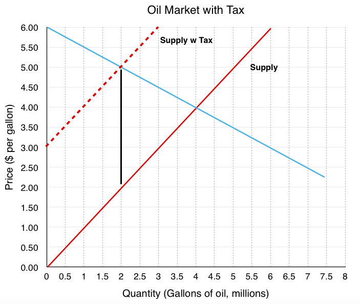
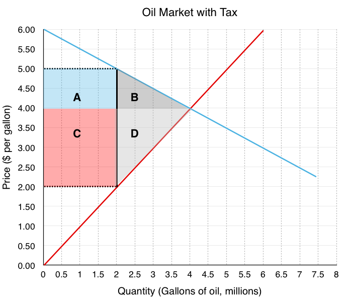
If the regime levies a $3 gas tax on producers (a legal revenue enhancement incidence on producers), the supply curve will shift upwards by $three. As shown in Figure 4.8a below, a new equilibrium is created at P=$v and Q=2 million barrels. Note that producers do non receive $5, they at present only receive $ii, as $iii has to exist sent to the government. From the consumer's perspective, this $one increment in price is no different than a price increment for any other reason, and responds by decreasing the quantity demanded for the college priced expert.
What if the legal incidence of the taxation is levied on the consumers? Since the demand curve represents the consumers' willingness to pay, the demand bend volition shift down as a outcome of the tax. If consumers are only willing to pay $4/gallon for 4 million gallons of oil just know they will confront a $3/gallon taxation at the till, they will only purchase 4 million gallons if the ticket cost is $1. This creates a new equilibrium where consumers pay a $2 ticket cost, knowing they will have to pay a $3 tax for a total of $5. The producers will receive the $2 paid before taxes.
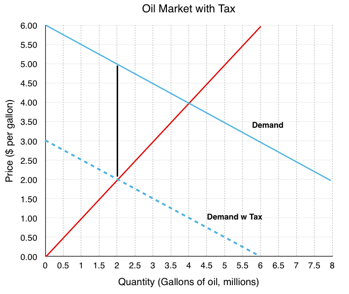
Note that whether the tax is levied on the consumer or producer, the final issue is the same, proving the legal incidence of the tax is irrelevant.
Tax – The Wedge Method
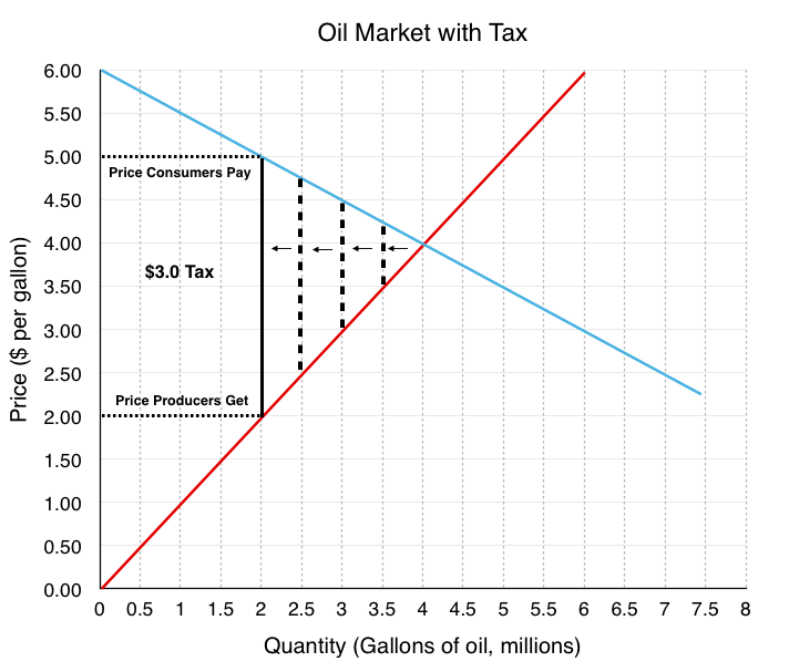
Another method to view taxes is through the wedge method. This method recognizes that who pays the tax is ultimately irrelevant. Instead, the wedge method illustrates that a tax drives a wedge between the price consumers pay and the revenue producers receive, equal to the size of the tax levied.
Equally illustrated below, to find the new equilibrium, ane simply needs to find a $3 wedge between the curves. The first wedge tested is simply $0.7, followed by $one.5, until the $3.0 tax is found.
Market Surplus
Like with price and quantity controls, 1 must compare the market surplus before and after a price modify to fully sympathise the furnishings of a taxation policy on surplus.
Before
The market surplus before the tax has not been shown, every bit the process should exist routine. Ensure you lot understand how to go the following values:
Consumer Surplus= $4 1000000
Producer Surplus = $8 meg
Market Surplus = $12 1000000
After
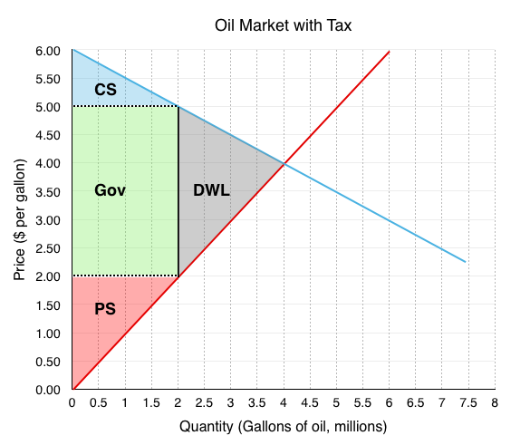
The market surplus afterwards the policy tin can be calculated in reference to Figure four.7d
Consumer Surplus (Blue Area) = $1 million
Producer Surplus (Carmine Area)= $2 million
Government Acquirement (Green Area) = $6 million
Market Surplus= $9 million
Why is Authorities Included in Marketplace Surplus
In our previous examples dealing with market place surplus, we did not include any give-and-take of authorities revenue, since the government was not engaging in our market. Remember that marketplace surplus is our metric for efficiency. If regime was not included in this metric, information technology would not be very useful. In this case a 1000000-dollar loss to government would exist considered efficient if information technology resulted in a $1 gain to a consumer. To ensure that our metric for efficiency is however useful we must consider regime when calculating market surplus.
Equally with the quota – both consumer and producer surplus decreased because of a reduced quantity. The divergence is, since the cost is irresolute, in that location is redistribution. This time, the redistribution is from consumers and producers to the authorities. Recollect, simply a alter in quantity causes a deadweight loss. Price changes simply shift surplus around between consumers, producers, and the government.
Transfer and Deadweight Loss
Let's look closely at the tax's touch on quantity and price to see how these components affect the market.
Transfer – The Bear upon of Cost
Due to the tax's effect on price, areas A and C are transferred from consumer and producer surplus to regime revenue.
Consumers to Government – Area A
Consumers originally paid $four/gallon for gas. Now, they are paying $five/gallon. The $1 increment in cost is the portion of the tax that consumers have to deport. Despite the fact that the tax is levied on producers, the consumers take to bear a share of the toll change. The size of this share depends on relative elasticity – a concept we will explore in the next section. This is because a subtract in price to producers means quantity supplied is falling, and in lodge to maintain equilibrium, quantity demanded must fall past an equal amount. This price change means the regime collects $i x 2 meg gallons or $2 meg in tax acquirement from the consumers. This is a straight transfer from consumers to government and has no result on market surplus.
Producers to Government – Area C
Originally, producers received revenue of $4/gallon for gas. Now, they receive $2/gallon. This $2 decrease is the portion of the taxation that producers take to bear. This ways that the government collects $2 x 2 million gallons or $4 million in tax acquirement from the producers. This is a transfer from producers to the regime.
As calculated, the government receives a total of $6 million in taxation revenue, which is taken from consumers and producers. This has no touch on on cyberspace marketplace surplus.
Deadweight Loss – The Touch on of Quantity
If we but considered a transfer of surplus, there would be no deadweight loss. In this example, though, nosotros know that cost changes come up with a change in quantity. A higher price for consumers will cause a subtract in the quantity demanded, and a lower cost for producers volition cause a subtract in quantity supplied. This reduction from equilibrium quantity is what causes a deadweight loss in the market since there are consumers and producers who are no longer able to buy and supply the practiced.
Consumer Surplus Decrease – Area B
Due to the increment in price, many consumers will switch abroad from oil to culling options. This subtract in quantity demand of ane.five one thousand thousand gallons of oil causes a deadweight loss of $1 million.
Producer Surplus Decrease – Area D
Producers, who now receive just $ii.00/gallon for their production, volition also subtract quantity supplied by 1.5 one thousand thousand gallons of oil. It is no coincidence that the size of the subtract is the aforementioned. When you create the wedge between consumers and producers, you lot are finding the quantity where the total amount of the taxation is incurred only the market is still at equilibrium. Recall that quantity demanded must equal quantity supplied or the market place will not be stable. This mirrored decrease in quantity ensures this is nevertheless the case. Notice, withal, that the impact of this quantity drop causes a larger subtract in producer surplus than consumer surplus totalling $2 million. Once more, this is due to elasticity, or the relative responsiveness to the cost gamble, which will exist explored in more detail shortly.
Together, these decreases cause a $3 million deadweight loss (the difference between the market place surplus before and market surplus after).
Subsidy
While a tax drives a wedge that increases the cost consumers have to pay and decreases the price producers receive, a subsidy does the opposite. Asubsidy is a do good given past the government to groups or individuals, usually in the grade of a cash payment or a tax reduction. A subsidy is often given to remove some type of burden, and it is frequently considered to be in the overall interest of the public. In economical terms, a subsidy drives a wedge, decreasing the toll consumers pay and increasing the price producers receive, with the government incurring an expense.
In Topic 3, we looked at a case study of Victoria'south competitive housing market where loftier demand drove upwards prices. In response, the regime has enacted many policies to allow depression-income families to nevertheless become homeowners. Let's wait at the effects of 1 possible policy. (Note the following policy is unrealistic only allows for easy comprehension of the result of subsidies).
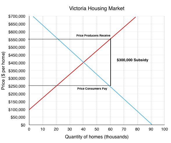
In the market higher up, our efficient equilibrium begins at a cost of $400,000 per home, with twoscore,000 homes being purchased. The government wants to essentially increase the number of consumers able to purchase homes, so it bug a $300,000 subsidy for any consumers purchasing a new home. This drives a wedge between what home buyers pay ($250,000) and what home builders receive ($550,000).
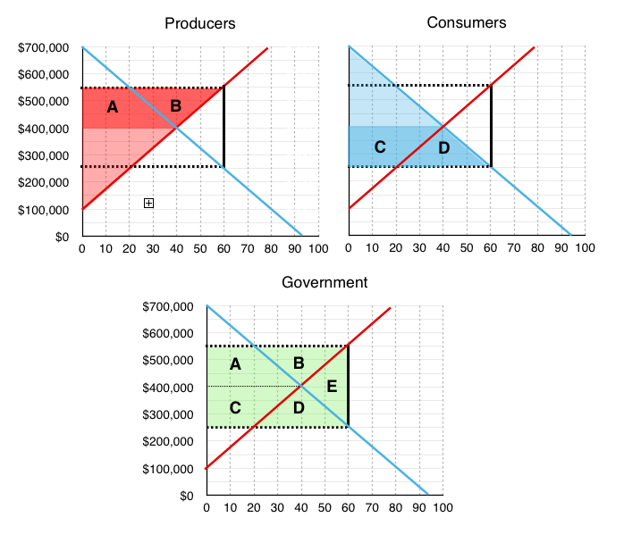
With all regime policies we have examined and then far, we have wanted to make up one's mind whether the result of the policy increases or decreases market place surplus. With a subsidy, we desire to do the aforementioned analysis. Unfortunately, because increases in surplus overlap on our diagram, information technology becomes more than complicated. To simplify the analysis, the post-obit diagram separates the changes to producers, consumers, and government onto different graphs.
Producers
The producers now receive $550,000 instead of $400,000, increasing quantity supplied to threescore,000 homes. This increases producer surplus byareas A and B.
Consumers
The consumers at present pay $250,000 instead of $400,000, increasing quantity demanded to 60,000 homes. This increases consumer surplus byareas C and D.
Government
The authorities now has to pay $300,000 per domicile to subsidize the 60,000 consumers buying new homes (this policy would cost the government $18 billion!!) Graphically, this is equal to a decrease in government to areas A, B, C, D and E.
Consequence
Our full gains from the policy (to producers and consumers) are areasA, B, C and D,whereas full losses (the toll to the authorities) are areasA, B, C, D, and Due east.To summarize:
AreasA, B, C and D are transferred from the government to consumers and producers.
Area Eastward is a deadweight loss from the policy.
There are two things to notice about this example. First, the policy was successful at increasing quantity from 40,000 homes to lx,000 homes. Second, information technology resulted in a deadweight loss because equilibrium quantity was too loftier. Remember,anytime quantity is changed from the equilibrium quantity, in the absence of externalities, there is a deadweight loss. This is true for when quantity is decreased and when it is increased.
http://www.investopedia.com/terms/s/subsidy.asp
Summary
Taxes and subsidies are more complicated than a cost or quantity control as they involve a third economic histrion: the regime. As we saw, who the tax or subsidy is levied on is irrelevant when looking at how the market ends upwards. Annotation that the last iii sections have painted a adequately grim flick about policy instruments. This is because our model currently does not include the external costs economic players impose to the macro-surroundings (pollution, disease, etc.) or attribute any meaning to equity. These concepts will be explored in more detail in later topics.
In our examples in a higher place, we see that the legal incidence of the revenue enhancement does not matter, but what does? To determine which party bears more of the brunt, we must use the concept of relative elasticity to our analysis.
Glossary
- Economic Tax Incidence
- the distribution of taxation based on who bears the burden in the new equilibrium, based on elasticity
- Legal Revenue enhancement Incidence
- the legal distribution of who pays the tax
- Subsidy
- a do good given past the government to groups or individuals, normally in the form of a greenbacks payment or a tax reduction It is ofttimes to remove some type of burden, and it is often considered to exist in the overall interest of the public
Exercises 4.7
Refer to the supply and demand curves illustrated below for the following Iii questions. Consider the introduction of a $20 per unit tax in this marketplace.
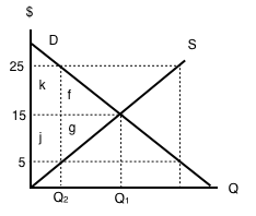
i. Which areas represent the loss to consumer AND producer surplus as a event of this revenue enhancement?
a) k + f.
b) j + grand.
c) k + j.
d) k + f + j + chiliad.
2.Which areas correspond the gain in government revenue as a result of this tax?
a) m + f.
b) j + one thousand.
c) k + j.
d) yard + f + j + g.
3. Which areas stand for the deadweight loss associated with this tax?
a) f + one thousand.
b) k – g.
c) j – f.
d) m + f + j + g.
4. Assume that the marginal cost of producing socks is constant for all sock producers, and is equal to $5 per pair. If government introduces a constant per-unit tax on socks, so which of the following statements is FALSE, given the after-revenue enhancement equilibrium in the sock market? (Presume a downward-sloping demand curve for socks.)
a) Consumers are worse off as a result of the tax.
b) Spending on socks may either increase or decrease as a result of the taxation.
c) Producers are worse off every bit a result of the tax.
d) This taxation volition result in a deadweight loss.
five. Refer to the supply and demand diagram below.
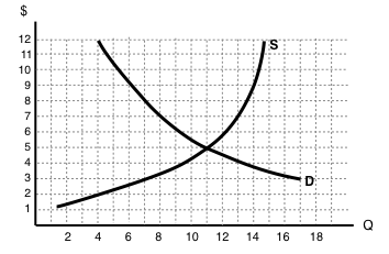
If an subsidy of $iii per unit of measurement is introduced in this market, the price that consumers pay volition equal ____ and the cost that producers receive net of the subsidy will equal _____.
a) $two; $five.
b) $3; $half dozen.
c) $iv; $seven.
d) $five; $8.
half dozen. If a subsidy is introduced in a market, so which of the post-obit statement is True? Assume no externalities
a) Consumer and producer surplus increase but social surplus decreases.
b) Consumer and producer surplus decrease but social surplus increases.
c) Consumer surplus, producer surplus, and social surplus all increase.
d) Consumer surplus, producer surplus, and social surplus all subtract
Use the diagram below to answer the following Two questions.
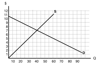
7. If a $six per unit of measurement tax is introduced in this market place, then the price that consumers pay will equal ____ and the toll that producers receive net of the tax will equal _____.
a) $10; $4.
b) $9; $3.
c) $8; $2.
d) $7; $i.
8. If a $six per unit taxation is introduced in this market place, then the new equilibrium quantity will exist:
a) 20 units.
b) twoscore units.
c) 60 units.
d) None of the higher up.
9. Which of the following statements about the deadweight loss of tax is TRUE? (Assume no externalities.)
a) If in that location is a deadweight loss, then the revenue raised by the tax is greater than the losses to consumer and producers.
b) If in that location is no deadweight loss, then revenue raised by the government is exactly equal to the losses to consumers and producers.
c) Both a) and b).
d) Neither a) nor b).
10. Which of the post-obit correctly describes the equilibrium effects of a per-unit of measurement tax, in a market with NO externalities?
a) Consumer and producer surplus increment but social surplus decreases.
b) Consumer and producer surplus decrease merely social surplus increases.
c) Consumer surplus, producer surplus, and social surplus all increase.
d) Consumer surplus, producer surplus, and social surplus all decrease.
xi. Which of the following correctly describes the equilibrium effects of a per unit subsidy?
a) Consumer price rises, producer cost falls, and quantity increases.
b) Consumer toll falls, producer price falls, and quantity increases.
c) Consumer price rises, producer price rises, and quantity increases.
d) Consumer price falls, producer price rises, and quantity increases.
12. Refer to the supply and demand diagram below.
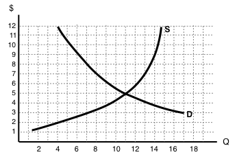
If an output (excise) tax of $5 per unit is introduced in this market, the price that consumers pay will equal ____ and the cost that producers receive net of the tax will equal _____.
a) $five; $10.
b) $6; $11.
c) $seven; $12.
d) $8; $three.
13. Consider the supply and demand diagram below.
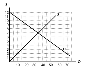
If a $2 per unit subsidy is introduced, what will be the equilibrium quantity?
a) 40 units.
b) 45 units.
c) 50 units.
d) 55 units.
Consider the supply and demand diagram below. Assume that: (i) in that location are no externalities; and (ii) in the absenteeism of regime regulation the market supply curve is the one labeled S1.
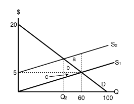
fourteen. If a $5 per unit of measurement taxation is introduced in this market, which area represents the deadweight loss?
a) a.
b) a + b.
c) b + c.
d) a + b + c.
Source: https://pressbooks.bccampus.ca/uvicecon103/chapter/4-6-taxes/
Post a Comment for "Forecasts Are More Accurate for Individual Items Than for Groups or Families of Items."